
Understand what considerations to take into account before attempting to interpret linear model results
The well-known linear regression model is probably one of the first tools in a data scientist’s pocket. Although perceived as “simple”, its potential shouldn’t be underestimated, especially if you’re interested in making predictions while also understanding what lies behind them. In fact, many researchers continue to use this great tool to make inferences through data in various commercial and scientific fields. Yet, in several cases, after spending some time trying to solve “real world problems’’, data scientists tend to relegate linear regression models, and shift their focus towards algorithms with stronger predictive power. Of course, the method selected should always depend on the problem at hand and the objective i.e. do you just want to answer “what” or do you also need to understand “how”?.
In any case, using linear regressions is not necessarily a simple task as it takes time, statistical knowledge, and non-linear processes (paradoxically) to process the data. It’s not just about running a script and validating certain hyper-parameters, you need to dig deeper.
In this short article we intend to present a summary of the main aspects and considerations to take into account when implementing a linear regression model. Note that this isn’t a prescription, it’s a guide to understand what to consider and where to pay attention before attempting to interpret results.
Applications
As we mentioned, one of the questions that we might be interested in answering is “how”. For example, understanding how the relationship between hours spent studying and test scores, education level and salaries comes to play; or maybe you own a business and are interested in understanding the marginal increase in sales for every dollar spent on a particular marketing campaign. Either way, you’ll notice that the key in each example is the word “understanding”, which can be interpreted as the understanding of the correlation between variables. In this context, a linear regression could be very useful to capture some interpretable patterns and “give” some ideas about what is happening behind the data.
As a refresher, when applying a linear regression, we assume that there is a certain “function or natural distribution” of the data that cannot be directly seen, but can be partially estimated using a set of characteristics from a sample of the population. In particular, this assumption involves many considerations that we should test and validate to be able to argue about the “veracity” of the results.
Example: Linear Regression model analysis in R
With that being said, let’s start with a practical example implemented in R, but first a brief context introduction.
Suppose that you plan to go fishing next weekend with some friends and you intend to surprise them by showing that you can estimate fish weights with very high precision just by using a tape measure. But that’s not all! you can also tell them how much the fish’s weight might change if any particular size measurement (vertical length, height, etc.) changes. So at this point, you may not be the most popular with your friends, but you could win some bets.
This is just a fun context to use our linear regression model and delve into advanced techniques. In this example, we will use a database of common fish species in the fish market that you can get from Aung Pyae in Kaggle. This dataset contains several columns that describe different measures of size and species, and has 158 observations. For this analysis, we will start by using 3 simple size measurement variables: vertical length, height, and diagonal weight (all variables in centimeters). These variables are the predictors of our model. For the response variable we have the weight in grams of the fishes. So now, let’s go fishing!
Importing packages
library(MASS)
library(Kendall)
library(car)
library(corrplot)
library(RColorBrewer)
Creating a function for plotting residuals
First of all, we’ll create a function that allows us to plot the residuals resulting from the regression model. In this case we take the studentized residuals since they perform better than the raw residuals when performing a later heteroscedasticity analysis. This is because the variance in the theoretical linear model is defined as “known”, and in the application the sample variance is estimated instead, so the raw residuals could show heteroscedasticity in the errors even when the residuals are homoscedastic. Here you can find a brief explanation about this effect.
plot_residuals = function(linear_model){
    res_stud=rstudent(linear_model)
    k=1
    for(i in res_stud){
      if(is.na(i)){res_stud[k]=0}
      else{res_stud[k]=i}
      k=k+1}
par(mfrow=c(1,2))
plot(linear_model$fitted.values,res_stud); abline(0,0); abline(-3,0,col="red"); abline(3,0,col="red")
qqnorm(res_stud); qqline(res_stud, col = 2)
}
Importing and exploring the dataset
We’ll initially use the variables vertical length, height and width of the fish as predictors, and the variable “weight” as the response variable.
df_fish = read.csv('Fish.csv',header=TRUE)
selected_cols = c('Weight','Length1', 'Height','Width')
df_fish = df_fish[,selected_cols]
attach(df_fish)summary(df_fish)
Delete rows with errors
After a brief review of the data, we found an observation with “weight” equal to 0 so we eliminate it to avoid future problems. In addition, it should be noted that the techniques for subsequently transforming the response variables and predictors require that the variables always take positive values.
df_fish = df_fish[Weight!=0,]
rownames(df_fish)=1:nrow(df_fish)
Exploring data
We continue with the data exploration by plotting a scatter diagram of the variables and a correlation matrix. Our aim here is firstly to find the existence of a correlation between the regressors and the response variable, and secondly to see the correlation between the predictor variables in anticipation of a possible multicollinearity problem.
# Scatter plot
par(mfrow=c(1,3))
pairs(df_fish)# Correlation matrix
M = cor(df_fish)
corrplot(M, type="lower",col=brewer.pal(n=8, name="RdYlBu"))

As we can see from the graphs, there seems to be a high correlation not only between the predictor variables and the response variable, but also between the predictors themselves. This means we’ll have to face the problem of multicollinearity.
Furthermore, the existence of a non-linear relationship between the predictors and the response variable can also be observed, which implies we’ll face structural problems in the residuals if we were to implement a linear model without any transformation of the variables.
In this regard, we’ll proceed to evaluate these inferences using tests and transformation techniques that will allow us to achieve a more precise correction of the model.
Train-Test split sample
We performed the training and test split using 80% and 20% of the observations, respectively.
n_sample = floor(0.8*nrow(df_fish))
set.seed(7)
train = sample(seq_len(nrow(df_fish)),size = n_sample)
train_sample = df_fish[train,]
row.names(train_sample) = NULL
test_sample = df_fish[-train,]
row.names(test_sample) = NULL
Model 1
Original linear model
We fit our first model using the 3 original predictors and the response variable. Then we print the results of the regression.
lm_original = lm(Weight~., data=train_sample)
summary(lm_original)

As we expected, the regression results show a good performance of the regressors. In fact, the model as a whole outperforms a model whose prediction consists of projecting the mean of the response variable (this difference is statistically significant at conventional values of confidence levels). We can observe this in the Fisher statistic with a p-value close to 0 and in the Adjusted R-squared, whose value indicates that the model explains 88% of the variability of the response variable around its mean.
In addition, when analysing the statistical significance of each variable within the model, we can see that the intercept, vertical length (Length1) and height of the fish are statistically significant at 1%, while the width variable of the fish is only significant at 10%.
Moreover, it is important to note that based on what we saw in the initial plot, we could have expected a higher correlation or significance level between the “weight” and the “width” of the fish. This difference between what we expected and what we found is due to what is called multicollinearity.
How can this be explained? The effect that we saw at the beginning would not correspond to the relationship between the variable “width” and the variable “weight”, but rather to the fact of this variable being strongly correlated with the variables “vertical length” and “height”. When looking at it isolated against the dependent variable it uses the information also reflected on the other variables to show its partial correlation. However, once we add the variables that directly affect the response variable, all this information is no longer captured by the “width”, reducing its explanatory power.
Checking multicollinearity
What’s the main problem with this phenomenon? Well, in presence of a very high correlation between the predictors, the explanatory effect of the variables is difficult to separate and in many cases distorts the values of the associated coefficients and their statistical significance. You must keep in mind that in most cases we can find that our explanatory variables are correlated with each other but the problem arises when this correlation is high. This is important if you are trying to make inferences and need to interpret the variables, whereas in the case of purely predictive models this is not relevant.
So, let’s see what happens with multicollinearity in this case. To do so, we’ll use the Variance Inflation Factor (VIF) since it allows us to understand the correlation of each predictor with respect to the other predictors (more details here) and helps us to define whether or not a variable can become a risk for our model.
There is no VIF value from which to determine that there is high or low multicollinearity, however, in practice it is considered that values close to 10 (or higher) for this index can be an indicator of multicollinearity, while values close to a 1 show very low multicollinearity.
vif(lm_original)

Observing the results we note a priori that there is a higher VIF associated with the variable “width”. As a result, we will reduce our model by eliminating the variable with the highest multicollinearity and we will recalculate the VIF with the remaining model.
Model 2
Reduced linear model
Now we fit our model again only with the variables “vertical length” and “height”.
lm_reduced = lm(Weight~Length1+Height, data=train_sample)
summary(lm_reduced)

The results of the model with the new subset of variables remain practically unchanged. What we can actually observe is a very small drop in the Adjusted R-squared with a very small increase in the mean square error, and a small improvement in the level of statistical significance of the variable “height”.
Checking multicollinearity
Let’s see what happens to the VIF of each predictor.
vif(lm_reduced)

As we can see, the VIF decreased significantly for the two remaining explanatory variables. This tells us that removing the variable “width” seems like a good decision (simpler is better).
Plotting residuals
Now that we have our variables defined, we proceed to perform a thorough analysis of the regression results.
In this process, the analysis of the residuals is a fundamental element to make the most of our regression model. To begin with, when using this type of model we start from the assumption of normality of the error distribution, and not just any type of normal distribution but one with mean 0. This is what allows us to take advantage of all the benefits that this model gives us in terms of inference.
We then perform an analysis of the residuals using the function to graph the studentized residuals described above.
plot_residuals(lm_reduced)

As we can see in the plot, there seems to be a kind of quadratic structure in the residuals and some outliers. This indicates that some additional information can still be extracted with the predictors used, but we will have to perform certain transformations on the variables to extract that information.
Regarding the normality of the data (Normal Q-Q Plot) we can observe some skewness and heavy tails of the distribution of the residuals compared to the theoretical quantiles of the normal distribution, so it is quite likely that the distribution of the errors does not have a normal distribution. In an attempt to validate this intuition we will use the Kolmogorov-Smirnov test, which allows us to compare, in general, whether two distributions are equal or not, and in this particular case, whether the distribution of the residuals is similar to the theoretical normal distribution with mean 0 and variance equal to the sample variance.
Testing normality in residuals
lm_reduced_residuals=rstudent(lm_reduced)
ks.test(lm_reduced_residuals,"pnorm",mean(lm_reduced_residuals),sd(lm_reduced_residuals))

The Kolmogorov-Smirnov test’s null hypothesis is that both distributions are not equal, while its alternative hypothesis is that both distributions are equal. Then, we would like to demonstrate that after running the test, the null hypothesis is rejected (we need a high p-value). However, in this case, we observe that the p-value is less than some of the conventional confidence levels, so we can say that (at the 1% level) we do not reject the null hypothesis and consequently we do not have sufficient evidence to suggest that both distributions are equal.
Heteroscedasticity: Testing correlation between residuals and fitted values
Next, we are interested in verifying the homoscedasticity of the residuals. By homoscedasticity we mean that errors do not grow or shrink as the values predicted by our model increase or decrease. This is a desired property in the construction of the model, as testing the absence of structure in the residuals, would indicate that there are no longer possible transformations of the currently used variables that could allow us to improve the performance of the model.
In this case, we need to show that there is some uniformity in the residuals and that they are scale invariant. Otherwise, we’ll be facing a loss of efficiency of the least squares estimators and the problems generated during the calculation of the matrix of variances and covariances of the estimators.
This is something that we can already observe in the previous plot. However, what we are aiming for is to be able to carry out a hypothesis test that allows us to validate the absence of correlation.
summary(Kendall(abs(lm_reduced$residuals),lm_reduced$fitted.values))

The applied test (Kendall’s test) is a correlation test similar to the Spearman test, which has some advantages in calculating the correlation coefficient (Tau in Kendall’s test, Rho in Spearman’s test). For more details go to the following link.
Kendall’s test indicates that the correlation coefficient (tau) between the residuals and the fitted values is positive (0.16) and statistically significant at 1%. This suggests that there is not enough evidence to support the hypothesis of absence of correlation, which means we are in a scenario with heteroscedastic residuals.
Model 3
Transforming the response variable
So, what do we do when we have structure in the residuals? We have two options that can help us reverse this problem: a) transforming the response variable and the second, b) transforming the predictors. There is no correct recipe to start carrying out the transformations, but in practice the usual thing is to start by transforming the response variable and reevaluate the results before proposing a new transformation.
Then, we will begin by transforming the variable “weight” using the Box-Cox maximum likelihood technic, since it allows us to estimate a lambda value to which the variable can be transformed as x power lambda (hopefully this will reduce the structure in the residuals). For more details go to the following link.
y_transformed=boxcox(lm_reduced)
y_transformed$x[which.max(y_transformed$y)]

The results suggest that a possible transformation on the variable “weight” would be to apply a lambda power = 0.38. Note that a transformation of this magnitude can complicate the interpretation of the final results of the model. In order to cope with this, in general, it is preferable to apply a transformation close to the suggested value that still allows us to interpret the coefficients with ease. For this reason, we choose a logarithmic transformation.
Running the linear model with the response variable transformed
lm_transform_y = lm(log(Weight) ~ Length1 + Height, data=train_sample)
summary(lm_transform_y)
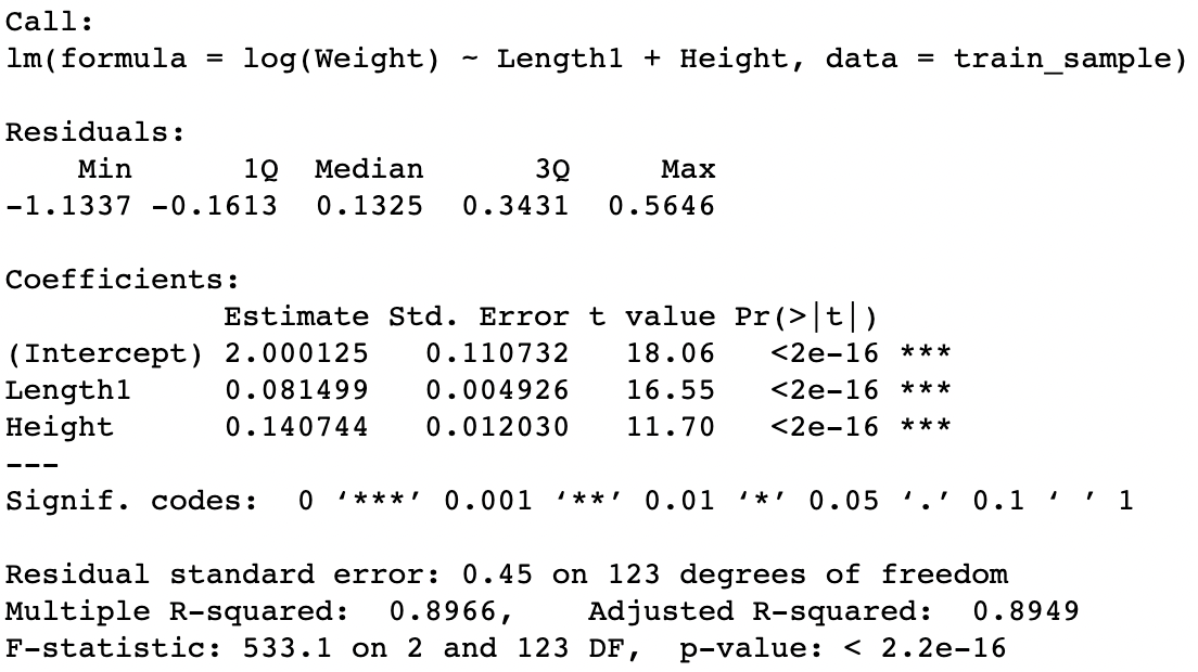
After applying this transformation, we notice a small but important improvement in the performance of the model. We can observe an increase of more than 1% of the Adjusted R Squared while maintaining the levels of statistical significance of both the model itself and the predictors. Regarding the error, it is important to highlight that now it is not comparable with the previous case since the response variable is on another scale.
Plotting residuals
plot_residuals(lm_transform_y)

So, did we solve the problem? When evaluating the structure of the errors, this first transformation not only seems to not have reversed the heteroscedasticity problem, but also appears to have “worsened” the distribution of the residuals, which is far from a normal distribution.
Let’s see what happens with the tests.
Testing normality in residuals
lm_transform_y_residuals=rstudent(lm_transform_y)
ks.test(lm_transform_y_residuals,"pnorm",mean(lm_transform_y_residuals),sd(lm_transform_y_residuals))

The distribution of the residuals moved farther away from the normal distribution, as we see reflected in the new p-value (current 0.01, previous 0.04). Therefore, we continue to reject normality in the error distribution.
Heteroskedasticity: Testing correlation between residuals and fitted values
summary(Kendall(abs(lm_transform_y$residuals),lm_transform_y$fitted.values))

Regarding heteroscedasticity, it also seems to have “worsened” although slightly, so we still cannot reverse this problem.
Model 4
Transforming the predictors
Then we move onto the transformation of the predictors. For this we will use the Box-Tidwell maximum likelihood transformation technique that will allow us to understand, like the Box-Cox transformation, what is the suggested lambda power to extract more information from the explanatory variables.
boxTidwell(log(Weight) ~ Length1 + Height ,data=train_sample)

The results obtained suggest applying a transformation of lambda = 0.007 for the variable Length1 and of lambda = -0.38 for the variable Height. In both cases, the suggested transformations are statistically significant at the 1% level, as indicated by the p-values of both variables. Consequently, we are once again in a scenario where making too precise transformations with respect to the suggested values could greatly complicate the subsequent interpretation of the results. Thus, we again choose to apply a logarithmic transformation to both variables.
Running the linear model with the response variable and predictors transformed
With these new transformations we proceed to adjust our linear regression model again.
lm_transform_y_X = lm(log(Weight) ~ log(Length1) + log(Height), data=train_sample)
summary(lm_transform_y_X)

As it can be seen, the transformations carried out as a whole produced a substantial improvement in the performance of the model, where the Adjusted-R-squared shows an increase of around 9% while maintaining the levels of statistical significance of both the model and the predictors.
Plotting residuals
plot_residuals(lm_transform_y_X)

When analysing the graphs of the residuals, we can also observe a notable improvement both in the reduction of the structure of the residuals and in the closeness to a normal distribution.
Testing normality in residuals
lm_transform_y_X_residuals=rstudent(lm_transform_y_X)
ks.test(lm_transform_y_X_residuals,"pnorm",mean(lm_transform_y_X_residuals),sd(lm_transform_y_X_residuals))

Finally, we have been able to reject the null hypothesis (p-value = 0.5!) so that, with the current model, there is not enough information to sustain that the distribution of the residuals is not normal. In practice, this tongue twister comes down to the fact that residuals can be considered normal.
Heteroscedasticity: Testing correlation between residuals and fitted values
summary(Kendall(abs(lm_transform_y_X$residuals),lm_transform_y_X$fitted.values))

Last but not least, we also found a significant reduction in the correlation between the residuals and the fitted values (0.01) with a high p-value (0.84) indicating that there is not enough evidence to even say that the little correlation that exists is statistically significant. So we reversed the problem of heteroscedasticity.
Results
Without further ado, here is our final model with its results.
As we have already mentioned, the performance of the model seems to be very good with a coefficient of determination (Adjusted R-squared) close to 99%, so that only with the variables “vertical length” and “height” we can explain almost all of the variation of the variable “weight”. In other words, our friends have no chance of beating us in the bets.
Also, as we highlighted, we well said that this type of model also allows us to infer the partial effect (we are not talking about causality in this case) of the predictors on the response variable, and thanks to the fact that the applied transformations were logarithmic functions, we can interpret the coefficients as a percentage variation of the explanatory variable. In other words, when the transformations build a log-log model (response variable in logarithms — predictors in logarithms) we have the possibility to interpret the partial correlations in terms of percentage rates of change.
In this way, the coefficient that accompanies the transformed variable log (Length1) is close to 2, which tells us that if instead of having caught the fish we just caught, we would have caught a fish whose length was 10% greater, the estimated weight of these fish would be about 20% greater than what we have now. Similarly, the coefficient that accompanies the transformed variable log (Height) is close to 1, which tells us that if instead of having caught the fish that we just caught, we would have caught a fish whose height was 10% greater , the estimated weight of this type of fish would also be around 10% more than what we have now.
This is great! We have converted our coefficients into a measure of elasticity between the dependent variable and each predictor. That’s right, we don’t even care about scale!
With this my friend, rest assured that you will become the king of nerdy fishing.
Conclusion
To sum up, this simple practical example allowed us to address numerous concepts and delve into linear regression models. The interesting thing is that, as in this toy example, many times linear models, no matter how simple they may seem, can have a very good performance and at the same time give us the possibility of obtaining very valuable insights from the results. Remember, the optimal answer to a question is not always the most complex one.