BNB post

A preview of Linear Programming’s capabilities to solve some business problems

Businesses (should) spend a lot of time and effort trying to predict the demand of their products/services, or the effort/resources required to complete different tasks so as to maximise their returns while avoiding mainly two undesirable outcomes:

• Falling short of resources or workers to cope with the demand, which could result in either processes failing or sales and client losses;
• Having way too many unused resources (overstocking) or unemployed workers, which means extra costs for storing goods and an opportunity cost in the case of the employees (maybe they could be assigned to other tasks).

Supposing a company has already managed to develop an accurate predictive model of their products/services’ demand, then the next step could be to organise the logistics behind their products replenishment and its tasks’ allocation in anticipation of the future demand. For example, this could mean finding an answer to the following questions:

i. From which warehouses is it cheaper to send the product “P” units that are expected to be sold within the next week/month, to each of my stores?

ii. How can I achieve this while taking into consideration the number of units available at each warehouse?

iii. What about the available transportation resources? How can I use my available vans/trucks to move the boxes of stock from warehouses to stores? What is the less costly option, considering that there’s a fixed limit of boxes that each van can transport?

iv. How can I assign the available workforce to each van while considering that some of my workers fought during a chess tournament last week and might end up fighting again if they are assigned to the same vehicle?

The question is then, how can one answer these types of questions that seem quite specific and different in nature? Well, we’d need to have a framework that allows us to build a fully customisable solution from scratch, where we can specify our objective and the real world constraints that define what is a feasible outcome of this objective. How about writing real life problems as systems of equations?

In this article, we’ll be simulating these scenarios and presenting a straightforward solution to the 4 questions proposed using a mathematical modelling approach known as Linear Programming. Though not in the data science spotlight, this is a famous optimisation technique/framework used to solve systems of linear equations that consist of an objective function (what we want to maximise/minimise, e.g. maximise profit while minimising costs), and a set of linear constraints that specify the different conditions that we need to meet in order to reach a feasible solution.

Basically, we write the problem we want to solve in linear terms specifying the objective and constraints, and then use optimisation algorithms (solvers) to navigate through thousands or millions of feasible and infeasible outcomes in a smart and efficient way, allowing us to at least come close to an optimal solution. But, what do we mean by optimal? In this framework optimal means the best feasible configuration of parameters that make up the final solution. Note that due to this, “optimal” may refer to completely different things depending on the business’ preferences/rules. For example, for one company satisfying the demand of their customers may be more important than saving transportations costs, while that may not be the case for others. At the end, it all comes to the correct specification of the business objective and its constraints.

A Problem, A Framework, A Solution

To answer the previous questions we’ll start by introducing a fictional setting. The context will be kept simple as the main aim of the article is just to introduce the framework and the idea of how we can use it to solve real life problems by developing custom solutions. Before starting, I’d like to clarify that the images/equations/code blocks that will appear from here onwards are all from my personal elaboration. Ok, let’s go straight to the point.

1. Context and sample results

Suppose you own a company, with a catalogue of 5 products (P=5), 3 warehouses (W=3), 3 stores (S=3), 4 vans (V=4) to transport the products and 8 employees (E=8) that can be assigned to each van in pairs (we can think that one is the driver and the other one the assistant). As mentioned at the beginning you already have an estimate of the expected demand. Furthermore, we’ll assume that due to the fact that you’ve estimated the demand, you’ve also stored enough stock to meet it, thus knowing how much stock you have in each warehouse.

To simplify the problem, instead of considering units of products, we’ll talk about boxes of products i.e. the demand and stock of a product is measured in boxes of the product (in a real life scenario after predicting the demand of products that are delivered in boxes/packages we’d need to convert the raw number into the number of boxes or grouping units needed as that’s the way of transporting them).

Next, we’ll assume you also know how much it costs to move a box of each product from any of your warehouses to any of your stores using any of your vans. Besides this variable cost, there’s also a fixed cost for using each vehicle (you can think of it as a depreciation/maintenance cost).

Additionally, we’ll suppose that there’s a limit to the number of trips each van can make. In this case the limit is 5 trips. What’s more, each van has a default number of boxes that it can fit in. On top of that, each of these vehicles (if used) needs to have employees assigned in pairs (a driver and an assistant) in order to be operational. Also, we can only assign each employee to a single van, and if we do, he’ll receive a fixed salary of $1500.

Finally, during a chess tournament that occurred the previous week, some of the employees got into a brawl so it is desirable to avoid assigning a pair of conflicting workers to the same van; as a matter of fact, we have 23 pairs of conflicting employees (J=23). If we do end up assigning them to the same van, we’ll have to deal with the consequences i.e. a penalty of $500.

In summary our context variables are the following:

• “P” products = 5
• “W” warehouses = 3
• “S” stores = 3
• “V” vans = 4
• “E” employees = 8
• “J” conflicting pairs of employees = 23

And the assumptions are:

• We know the demand in boxes of each of our products, by store;
• We know how many boxes of our products are available in each of our warehouses;
• All the boxes have the same size (to simplify the problem);
• We know how many boxes fit in each of the vehicles;
• The cost of sending a box varies depending on the combination of product-warehouse-store-van;
• The use of each van has a fixed cost;
• The vans can’t go from a warehouse to a store without transporting at least 1 box;
• The vans can’t do more than 5 trips. We can assume that they all occur on the same day;
• There’s a limit to how many boxes can be transported by each van;
• None of the vans can repeat the same trip;
• We need 2 employees assigned per van to be able to make a trip;
• If we assign an employee we have to pay him for this task 🙂;
• Each employee can only be assigned to a single van;
• It is desirable to avoid assigning conflicting employees to the same vehicle.

Then, the problem we have to solve is finding the optimal (less costly) way of transporting product boxes from warehouses to stores employing different vans and workers while fulfilling the constraints of demand, stock, vans and workers assignment.

The results look like this:

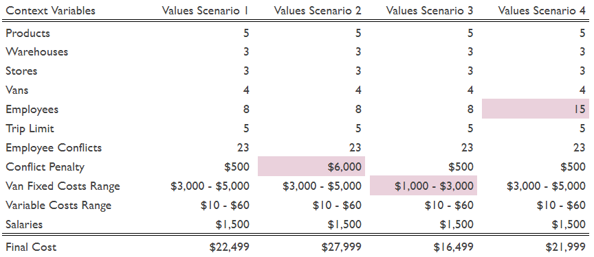
This table illustrates the results obtained (final cost) in different scenarios with partial variations in some parameters (conflict penalty, van fixed costs and number of employees). Note that the possibility of experimenting with different parameters is one of the main strengths of this framework. Of course, the analysis would be richer if we tried several changes at once such as allowing the vans to make more trips while reducing the penalty costs and increasing the number of conflicts. In fact, I encourage you to try some of these changes later.

Ok, from now on things will get a little more technical…

2. Variables, objective and constraints

The first thing we need to establish are the variables that we are going to use in the system of equations that define the problem. Here’s a list of them, with their description and range of values:

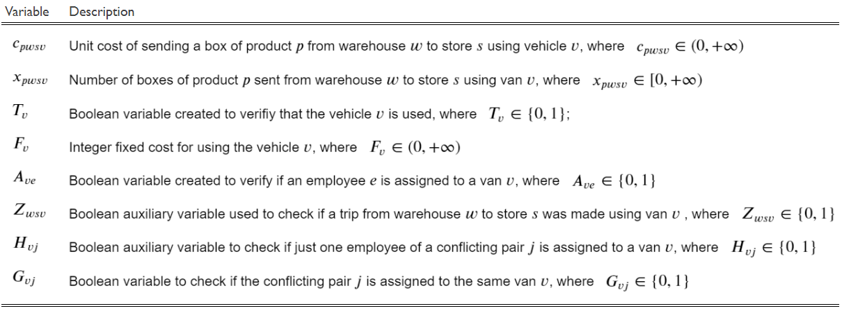
Now that we’ve specified the variables, we’ll write the problem. In mathematical terms, the problem to solve is the following:

i) The objective

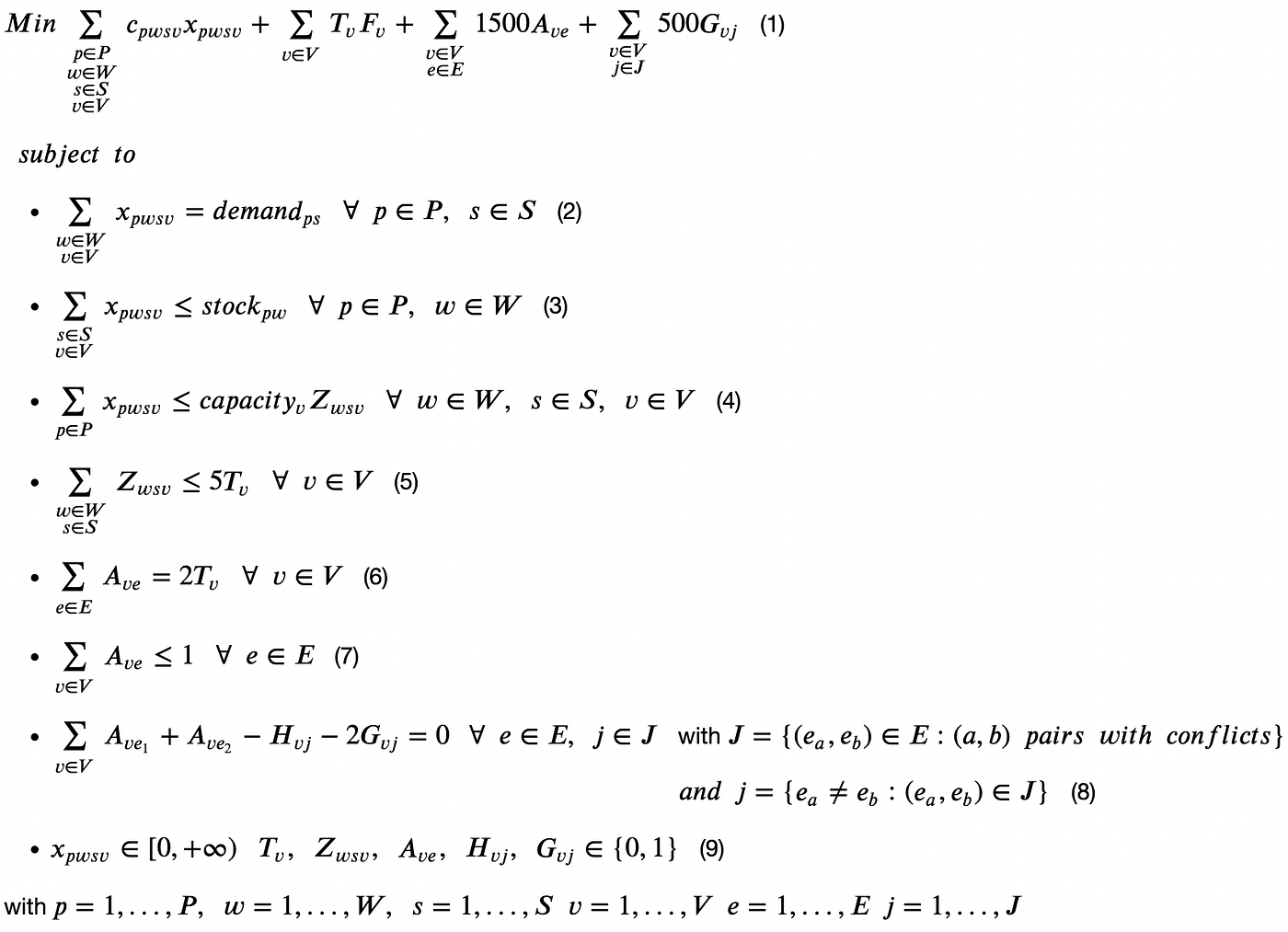
(1) This is the objective function represented as the sum of four terms: a) the sum of unit costs times the number of boxes of product p sent from warehouse wto store s using van v; b) the sum of fixed costs F of the vans used; c) the sum of the salaries of the employees e assigned to van v; d) the penalty cost for not complying with the optional constraint of not assigning the conflicting pair of employees j to the same van v.

ii) The constraints

(2) The first restriction specifies that the demand of each product p at each store s must be satisfied, i.e. the sum of all the combinations of product boxes sent from each warehouse w to each store s using any of the vehicles v must equal the number of boxes needed by the store to cover their expected demand;

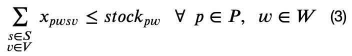
(3) Stipulates that we can’t send boxes that we don’t have. In other words, the sum of product boxes sent from a warehouse must be lower or equal than its available boxes;

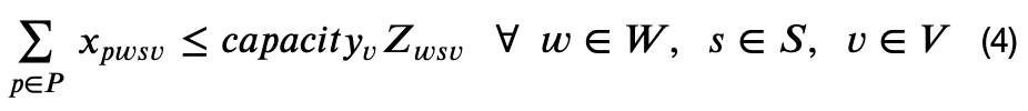
(4) Specifies that we can’t surpass the limit of boxes that can fit the van, so the sum of boxes transported in each vehicle must be lower or equal to the van’s capacity (capacity_v) at each trip. With this constraint we count the number of trips a van will make with the auxiliary variable Z_wsv, as capacity_v is the maximum number of boxes that can be transported at each trip by vehicle v, we can count as one trip the transportation of several products. Also, this constraint implicitly blocks the possibility of repeating the same trip;

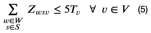
(5) Signals that none of the vans can make more than 5 trips while also checking if each of them was used or not. Note that this constraint is chained with the previous one. How? Well, once we know if a trip was made or not by using constraint (4), we simply sum the number of Z_wsv and require that the total is lower or equal than 5 (the trip limit). Here, due to the specification of the equation, T_v will be equal to 1 unless the van is left unused;

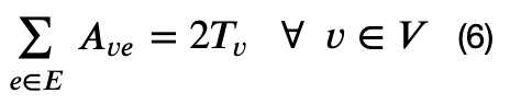
(6) Specifies that each van will have 2 or zero employees assigned;

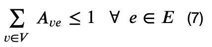
(7) Requires that each employee can only be assigned to a single van;

(8) This constraint accounts for the fact that the desirable constraint on the pair of conflicting employees j is optional. When a pair of conflicting employees j=(e1, e2) is assigned to the same van (A_ve1 + A_ve2 = 2) then the penalty is activated (G_vj=1) so that the equation equals zero. If just one member of the pair is assigned to a van then H_vj=1. If none of the conflicting employees of pair j is assigned to the van v then all the elements are zero.

(9) The final constraint specifies the upper and lower bound for each variable. Here we declare which variables are binary and which ones are integers.

The complete problem is then expressed as:

Since we’ve already managed to write the problem, we can proceed to code the solution of these examples using Google OR-Tools with Python. But, before proceeding it is important to highlight that taking your time to complete the previous step is quite relevant, as it will allow you to get a better grasp of the problem at hand, while potentially avoiding some future bugs in your code and helping you explain your reasoning to your fellow data science teammates.

3. Solution

You can check the whole solution in this notebook.

First, we import the packages we’ll be using for this example.

import numpy as np
import pandas as pd
from ortools.linear_solver import pywraplp

The solution consists of the following steps:

1. Set a seed to be able to replicate the simulation;
2. Declare the number of warehouses, products, stores, vans, employees and trip limit;
3. Set some thresholds for the simulated data and values for the fixed salary and the penalty for assigning a pair of conflicting employees to the same van;
4. Generate the matrices of costs (1 per product), the stock vector (1 per product, showing its stock available at each warehouse), the demand vector (1 per product, showing its demand at each store), a list of capacity per van (how many boxes each of them can transport per trip) and finally, the list of pairs of conflicting employees;
5. Call an instance of a solver that can be used to find a solution to the type of problem at hand (Integer Programming or Mixed Integer Programming);
6. Create the variables;
7. Define the constraints;
8. Define the objective function and the problem (maximisation/minimisation);
9. Solve and verify that the results comply with the constraints.

We start with steps 1–4. As we are simulating the problem, the costs and quantities are created with a random variable, but in a real scenario we’d need to use the inputs given by the business. The process looks like this:

https://towardsdatascience.com/media/4e4aca2f4c09530c0f012108261a1853

Now, to complete step 5 we need to instantiate a solver. In this case, we are using pywraplp from Google OR-Tools. Note that there are several solvers available in pywraplp such as GLOP, SCIP, GUROBI and IBM CPLEX. Since GUROBI and CPLEXrequire a licence and GLOP is designed for simple Linear Programming but the problem we have at hand requires a solver to approach Integer or Mixed Integer Linear problems, we’ll use SCIP (one of the fastest non-commercial solvers that can handle Integer and Mixed Integer Linear problems).

solver = pywraplp.Solver.CreateSolver('SCIP')

After that, we continue with step 6 i.e. the definition of the variables that make up the system of linear equations.

First, for each combination of product, warehouse, store and van, we need to create an x variable with indices p(product), w(warehouse), s(store), v(van) that tells us the integer number of boxes of product p sent from warehouse w to store s using van v. These integer variables (solver.IntVar) are restricted to positive numbers (lower bound = 0 and upper bound = solver.infinity()). Furthermore, to keep track of each specific variable and future constraints, we carefully name them. An example of one of these variables is x_1_1_1_1.

x = {}
for p in range(P_products):
  for w in range(W_warehouses):
    for s in range(S_stores):
      for v in range(V_vans):
        x[p,w,s,v] = solver.IntVar(lb=0,
                                  ub=solver.infinity(),
                                  name=f"x_{p+1}_{w+1}_{s+1}_{v+1}")

Second, we generate the boolean variable (solver.BoolVar) T_v that tells us if van v is used, which is required to be able to assign a cost for its usage.

T = {}
for v in range(V_vans):
  T[v] = solver.BoolVar(name=f"T_{v+1}")

Third, we create variable A_ve, which signals if employee e is assigned to van v. We need to do this in order to be able to consider the cost of the work of the employees.

A = {}
for v in range(V_vans):
  for e in range(E_employees):
    A[v,e] = solver.BoolVar(name=f”A_{v+1}_{e+1}”)

Fourth, we generate the variable Z_wsv, an auxiliary boolean variable used to count the number of trips a van makes. Each of them will tell us if the trip from warehouse w to store s was assigned to van v.

Z = {}
for v in range(V_vans):
  for w in range(W_warehouses):
    for s in range(S_stores):
      Z[w,s,v] = solver.BoolVar(name=f”Z_{w+1}_{s+1}_{v+1}”)

Lastly, we generate variables H_vj and G_vj. H_vj signals that just 1 of the conflicting employees of the conflicting pair j was assigned to van v. Variable G_vj signals that both members of a pair of conflicting employees j were assigned to van v.

H = {}
G = {}
for v in range(V_vans):
  for j in range(len(J_employees_conflicts)):
    H[v,j] = solver.BoolVar(name=f"H_{v+1}_{j+1}")
    G[v,j] = solver.BoolVar(name=f"G_{v+1}_{j+1}")

After creating the variables, we proceed to generate the linear constraints (we use the method solver.Add to do this). Regarding the demand constraints, we declare that the sum (solver.Sum) of the stock sent from each warehouse must equal the store’s demand. In the case of the stock constraints, we specify that the sum of the stock sent to each store must be lower or equal to the available stock at each warehouse. In both cases we use the function product from the library itertools to obtain the cartesian product of possible combinations (warehouses, vans) and (stores, vans).

# Demand constraint
for p in range(P_products):
  for s in range(S_stores):
    solver.Add(
    solver.Sum(
    [x[p, j[0], s, j[1]] for j in itertools.product(
                                  range(W_warehouses),
                                  range(V_vans))]) == demands[p][s],
                                  name='(2) Demand')# Stock constraint
for p in range(P_products):
  for w in range(W_warehouses):
    solver.Add(
    solver.Sum(
    [x[p, w, j[0],j[1]] for j in itertools.product(
                                   range(S_stores),
                                   range(V_vans))]) <= stocks[p][w],
                                   name='(3) Stock')

Note that we added a name to each restriction using the parameter “name”. This will allow us to identify them in the standard problem representation (LP format) using the function solver.ExportModelAsLpFormat, which I strongly advise you to use:

print(solver.ExportModelAsLpFormat(obfuscated=False))

Here’s a snapshot of how the constraints look like:

This is a sample of the demand and stock constraints (remember that x takes the form x_pwsv). The first one, as requested, shows that the number of boxes of product p=5 sent from any warehouse w to store s=3 using any van v must equal the demand=3 of store 3, which was generated before using a random variable. The stock constraint shows that the number of boxes of product p=1, sent from warehouse w=1 to any of the stores s, using any of the vans v must be lower or equal to stock=11, the randomly generated stock of product 1 for warehouse 1. The rest of these specific constraints follow the same logic.

Next, we add the trip and vans’ use constraints. With the first one we ask that none of the vans can transport more boxes than its capacity allows per trip, while also checking if a trip from warehouse w to store s was assigned to van v. The second constraint aids us to verify if van v was used.

# Trip verification constraint
for v in range(V_vans):
  for s in range(S_stores):
    for w in range(W_warehouses):
      solver.Add(
      solver.Sum(
      [x[p, w, s, v] for p in range(P_products)])
      <= capacities[v]*Z[w, s, v],
      name='4) TripVerification')# Van use and trip limit constraint
for v in range(V_vans):
  solver.Add(
  solver.Sum(
  [Z[j[0], j[1],v] for j in itertools.product(
                            range(W_warehouses),
                            range(S_stores))]) <= trip_limit*T[v],
                            name='5) TripLimit')

Let’s see a sample of how these constraints look like:

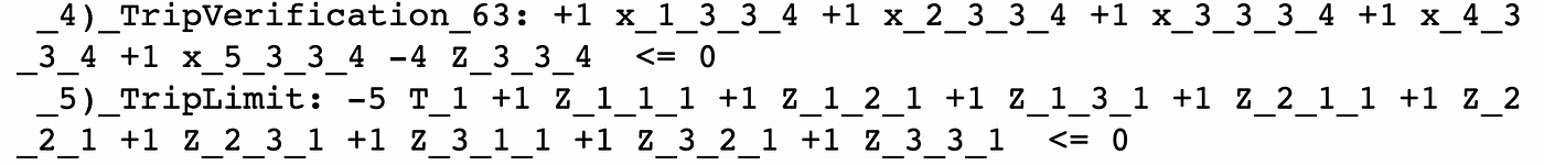
On one hand, constraint TripVerification_63 checks if van v=4 was assigned to go from warehouse w=3 to store s=3. Note that the term Z_wsv is multiplied by 4, which is the capacity of van v. This means that to comply with the constraint, the highest sum of quantities transported can’t be greater than 4. Also, in any case, for all quantities higher than 0, Z_wsv must equal 1. And that’s how we verify if a trip was assigned to be done.

On the other hand, the example of the TripLimit constraint implies that the sum of all possible trip paths (w_s) of van v=1, must be lower or equal to 5 (the trip limit that we set at the beginning) as we have the term of -5T_1. Note that this last term will also tell us if van v=1 will be used. The same logic is applied to the rest of the vans in the remaining constraints of this class.

After this, we follow up with the final constraints: (6) EmployeeRequirement,(7)JobLimit and (8) ConflictVerification. With EmployeeRequirement we ask that for a van to be used, it must have two employees assigned. Next, JobLimit implies that we can’t assign an employee to more than 1 van. And finally, ConflictVerification is built to verify whether or not each pair of the J employee conflicts is assigned to the same van.

# Number of employees per van
for v in range(V_vans):
  solver.Add(
  solver.Sum(
  [A[v,e] for e in range(E_employees)]) == 2*T[v],
  name='6) EmployeeRequirement')# Number of vans an employee can be assigned to
for e in range(E_employees):
  solver.Add(
  solver.Sum([A[v,e] for v in range(V_vans)]) <=1,
  name='7) JobLimit')# Verification of the constraint compliance
for v in range(V_vans):
  for idx,j in enumerate(J_employees_conflicts):
    solver.Add(
    solver.Sum([A[v,j[0]-1]])==-A[v,j[1]-1]+H[v,idx]+2*G[v,idx],
    name='8) ConflictVerification')

A sample of the first two would be:

Both constraints are straightforward. EmployeeRequirement_69 tells us that for van v=4 to be used, we need to have at least 2 employees assigned to it. JobLimitspecifies that employee e=1 can be assigned to just 1 van.

Regarding the last constraint, probably the hardest one to understand, we have 2 examples:

ConflictVerification_152 checks if the conflicting pair of employees j=8, composed of employees e=2 and e=3 is assigned to van v=4. If just 1 of these employees is assigned to it, then H_4_8 must equal 1 for the equation to equal 0. If both employees are assigned to this van, then G_4_8 must equal 1 for the equation to equal 0. Note that only the second case would have an impact on the total cost as the penalty of $500 would be activated. In the case of ConflictVerification_152, we can directly see that it checks the exact same thing but for conflicting pair j=9, composed of employees e=2 and e=4.

Since we’ve finished writing the series of constraints, we are ready to continue with step 8 i.e. the definition of the objective function and the type of problem (maximisation/minimisation). To do so, we first create a list to save each of the terms described before as the objective function is simply the sum of all of them. Then, after adding all the terms we specify that we want to solve a minimisation problem (solver.Minimize).

# Objective Function
objective_function = []# First term -> Transportation variable costs
for p in range(P_products):
  for w in range(W_warehouses):
    for s in range(S_stores):
      for v in range(V_vans):
        objective_function.append(costs[p][w][s][v] * x[p, w, s, v])# Second term -> Transportation fixed costs
for v in range(V_vans):
  objective_function.append(costs_v[v]*T[v])# Third term -> Salary payments
for v in range(V_vans):
  for e in range(E_employees):
    objective_function.append(fixed_salary*A[v,e])# Fourth term -> Penalties for not avoiding conflicts
for v in range(V_vans):
  for j in range(len(J_employees_conflicts)):
    objective_function.append(conflict_penalty*G[v,j])# Type of problem
solver.Minimize(solver.Sum(objective_function))

Here’s the whole objective function, where all variables are binary except for x, that is an integer:

Finally we use the Solve method to run the optimisation algorithm.

# Call the solver method to find the optimal solution
status = solver.Solve()

All that’s left is checking the solution. To do this we call the solution status, if it is optimal (pywraplp.Solver.OPTIMAL) we print the value of the objective function, if that’s not the case we should check our previous work and look for inconsistencies in the problem definition.

if status == pywraplp.Solver.OPTIMAL:
  print(
   f'\n Solution: \n Total cost = ${solver.Objective().Value()}'
   )
else:
    print(
    'A solution could not be found, check the problem specification'
    )

For this simulation, the solution is:

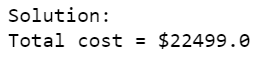
This means that the optimal transportation of products from warehouses to stores using vans, ends up costing $22,499. Now we have to decide whether or not this is good enough. If we think we can find a better solution by modifying the definition of the problem, we should think of how we can add/remove or modify some of the constraints or, if possible, how to alter the context variables. If we believe this is ok, then the next natural step would be to check the optimal values of the variables of the model, as from a planning perspective, it is highly relevant to be able to tell which are the vans that are going to be used, who are the employees that are going to be working in these tasks; which of them are assigned to which van; which are the trips that need to be planned and the quantity and types of products transported at each of them.

For the sake of finishing this article, we’ll just assume that there’s nothing left to do so we can proceed to check the optimal values of the relevant variables by extracting the solution details.

4. Fleet and workforce planning details

To begin the extraction of useful details we follow a simple procedure: i) extract the optimal values for each variable; ii) preprocess and rearrange the data into a table; iii) query the table with different filters. Here’s i) and ii):

result_list = []# Extract the solution details and save them in a list of tables
for var in [x,Z,T,A,H,G]:
  variable_optimal = []
    for i in var.values():
      variable_optimal.append(i.solution_value())
    
      var_result=list(zip(var.values(),variable_optimal))
    
      df=pd.DataFrame(var_result,columns=['Name','Value'])
    
      result_list.append(df)# Concatenate the tables and extract the variable names
results=pd.concat(result_list)
results['Name']=results['Name'].astype(str)
results.reset_index(drop=True,inplace=True)
results['Variable']=results['Name'].str.extract("(^(.)\d?)")[0]
results['Variable']=results['Variable'].str.upper()
results['Value']=results['Value'].map(int)# Create a mapping of variables and indices to simplify the analysis
variable_indices={'X':'X_product_warehouse_store_van',
                  'A':'A_van_employee',
                  'T':'T_van',
                  'H':'H_van_pair',
                  'G':'G_van_pair',
                  'Z':'Z_warehouse_store_van'}results['Indices']=results['Variable'].map(variable_indices)# Order the columns
results=results[['Variable','Indices','Name','Value']].copy()

This would be a sample of the main table:

Next, after creating our main dataframe, we look for the vans that we are going to use by filtering the column Variable with “T” (binary variable to signal the usage of the vehicle) and the column Value with 1 (which means, the optimal solution implies that we need to use these vans):

list(results[(results[‘Variable’]==’T’)&(results[‘Value’]==0)].Name)

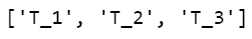
The results show that vans 1, 2 and 3 will be used.

For the next part, we’ll just search for the variables related to van 1, starting with answering which trips are going to be made using this vehicle. Here it is important to remember that van v=1 corresponds to the index v=0:

trips_van_1=[]
for w in range(W_warehouses):
  for s in range(S_stores):
    for v in range(V_vans):
      if v==0:
        trips_van_1.append(str(Z[w,s,v]))trips_df=results[(results['Variable']=='Z')&(results['Value']>0)]display(trips_df[trips_df['Name'].isin(trips_van_1)])

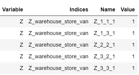
We can see that van 1, is assigned the following 5 trips:

• Warehouse 1 to store 1 and 3;
• Warehouse 2 to store 2;
• Warehouse 3 to store 2 and 3;

Next, we need to find the employees that are going to be in charge of the delivery operations of van 1:

employees_van_1=[]
for v in range(V_vans):
  for e in range(E_employees):
    if v==0:
     employees_van_1.append(str(A[v,e]))
            
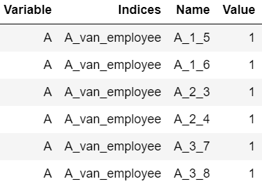
employees_df=results[(results['Variable']=='A')&(results['Value']>0)]display(employees_df[employees_df['Name'].isin(employees_van_1)])

This table tells us that employees 5 and 6 are the ones assigned to the van. Now the final question regarding van 1 is how many boxes and of which products it will have to transport at each of the trips. Let’s do this for the trip from warehouse 2 to store 2:

transport_df = results[(results['Variable']=='X')&(results['Value']>0)]transport_trip_2_2 = []for p in range(P_products):
  for w in range(W_warehouses):
    for s in range(S_stores):
      for v in range(V_vans):
        if w==1 and s==1 and v==0:
          transport_trip_2_2.append(str(x[p,w,s,v]))display(transport_df[transport_df['Name'].isin(transport_trip_2_2)])

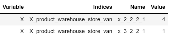
So, during the trip from warehouse 2 to store 2, van 1 will transport 5 boxes (its maximum capacity), 4 of product 2 and 1 of product 3. Note that during these examples we verified that the model is working as intended i.e. constraints were taken into consideration to obtain the optimal solution. To wrap up, we just need to check what happened with the constraint for the conflicting pair of employees:

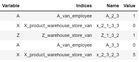
results[(results['Variable']=='G')&(results['Value']!=0)]

Well, it looks like the pair of conflicting employees j=14 (employees 3 and 4) was assigned to van 2 in the optimal solution. If that’s the case, then A_2_3 and A_2_4 should be equal to 1, let’s check it:

results[(results['Variable']=='A')&(results['Value']!=0)]

And with that, we finally finished with the examples.

Concluding Remarks

All in all, we’ve seen that it is indeed possible to write real life problems as systems of linear equations. What’s more, we are also able to solve them. Of course, finding an optimal solution strictly depends on the context variables, the objective and the set of constraints. However, a really complex setting may make finding an optimal solution a much harder process, as more combinations of parameters would need to be analysed, which in turn would require more computing power.

Finally, even though the example provided in this article relates to a fleet and workforce planning problem, the applications of this framework are much broader. Strictly speaking, I’ve employed this approach to solve problems related to Logistics, Supply Chain Management and Pricing and Revenue Management, but the possible applications go quite further as it is also frequently used to solve problems related to Health Care Optimisation, Urban design, Management Scienceand Sports Analytics.

For those who arrived at this point, I hope you were able to obtain some insights to build your own solutions. And don’t worry, even though arguably the hardest part is to define the problem, once you do it, the next steps are quite straightforward. Thanks for reading!

References

[1] Linear Programming: Foundations and Extensions (International Series in Operations Research & Management Science Book 285)